
Pandas from Numpy#
This tutorial will show the fundamental structure of Pandas Data Frames. We will look at the components that constitute a Data Frame - for instance, Numpy arrays - in order to gain a deeper understanding of the raw ingredients that more advanced Pandas methods and functions operate on.
What is Pandas?#
Pandas is an open-source python library for data manipulation and analysis.
Note
Why is Pandas called Pandas?
The “Pandas” name is short for “panel data”. The library was named after the type of econometrics panel data that it was designed to analyse. Panel data are longitudinal data where the same observational units (e.g. countries) are observed over multiple instances across time.
The Pandas Data Frame is the most important feature of the Pandas library. Data Frames, as the name suggests, contain not only the data for an analysis, but a toolkit of methods for cleaning, plotting and interacting with the data in flexible ways. For more information about Pandas see this page.
The standard way to make a new Data Frame is to ask Pandas to read a data file
(like a .csv file) into a Data Frame. Before we do that however, we will
build our own Data Frame from scratch, beginning with the fundamental building
block for Data Frames: Numpy arrays.
# Import the libraries needed for this page
import numpy as np
import pandas as pd
Numpy arrays#
Let’s say we have some data that applies to a set of countries, and we have some countries in mind:
country_names_array = np.array(['Australia', 'Brazil', 'Canada',
                                'China', 'Germany', 'Spain',
                                'France', 'United Kingdom', 'India',
                                'Italy', 'Japan', 'South Korea',
                                'Mexico', 'Russia', 'United States'])
country_names_array
array(['Australia', 'Brazil', 'Canada', 'China', 'Germany', 'Spain',
       'France', 'United Kingdom', 'India', 'Italy', 'Japan',
       'South Korea', 'Mexico', 'Russia', 'United States'], dtype='<U14')
For compactness, we’ll also want to use the corresponding standard three-letter code for each country, like so:
country_codes_array = np.array(['AUS', 'BRA', 'CAN',
                                'CHN', 'DEU', 'ESP',
                                'FRA', 'GBR', 'IND',
                                'ITA', 'JPN', 'KOR',
                                'MEX', 'RUS', 'USA'])
country_codes_array
array(['AUS', 'BRA', 'CAN', 'CHN', 'DEU', 'ESP', 'FRA', 'GBR', 'IND',
       'ITA', 'JPN', 'KOR', 'MEX', 'RUS', 'USA'], dtype='<U3')
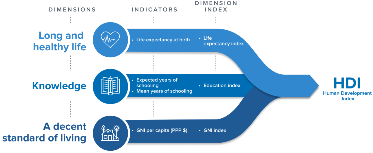
For each of these countries, we have a Human Development Index (HDI) score. The HDI score for a country is a summary over multiple dimensions of human development: life expectancy, average years of schooling and Gross National Income per capita.
# Human Development Index Scores for each country
hdis_array = np.array([0.896, 0.668, 0.89,
                       0.586, 0.89,  0.828,
                       0.844, 0.863, 0.49,
                       0.842, 0.883, 0.824,
                       0.709, 0.733, 0.894])
hdis_array
array([0.896, 0.668, 0.89 , 0.586, 0.89 , 0.828, 0.844, 0.863, 0.49 ,
       0.842, 0.883, 0.824, 0.709, 0.733, 0.894])
By the way, these data are real; they come from statistics compiled by the United Nations. For simplicity, we are only looking at data from the year 2000. See the datasets and licenses page for more detail.
Let’s say we also have the fertility rate for each country. The fertility rate is the average number of children born to to each woman. In due course, we’re interested to see whether HDI can predict the fertility rate values.
# Fertility rate scores for each country
fert_rates_array = np.array([1.764, 2.247, 1.51,
                             1.628, 1.386, 1.21,
                             1.876, 1.641, 3.35,
                             1.249, 1.346, 1.467,
                             2.714, 1.19 , 2.03 ])
fert_rates_array
array([1.764, 2.247, 1.51 , 1.628, 1.386, 1.21 , 1.876, 1.641, 3.35 ,
       1.249, 1.346, 1.467, 2.714, 1.19 , 2.03 ])
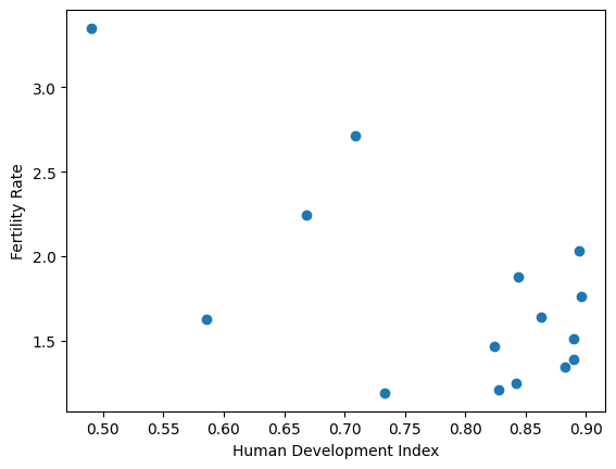
As experienced data analysts, we first want to inspect this relationship graphically, for example with the Matplotlib library. Later, we will see that Pandas offers us some streamlined ways of plotting data, without the need to import other libraries.
# Some basic plotting with Matplotlib.
import matplotlib.pyplot as plt

plt.scatter(hdis_array, fert_rates_array)
plt.xlabel('Human Development Index')
plt.ylabel('Fertility Rate');
Pandas Series (aka an array + an index)#
(Aka is an abbreviation for “Also Known As”.)
We want a good way to keep it clear which value corresponds to each country. We’re going to start with the HDI values.
One way of doing that is to make a new data structure that contains the HDI values, but also has labels for each value. Pandas has an object for that, called a Series. You can construct a Series by passing the values and the labels:
# Make a Series from the `hdis_array`
hdi_series =  pd.Series(hdis_array, index=country_codes_array)
hdi_series
AUS    0.896
BRA    0.668
CAN    0.890
CHN    0.586
DEU    0.890
ESP    0.828
FRA    0.844
GBR    0.863
IND    0.490
ITA    0.842
JPN    0.883
KOR    0.824
MEX    0.709
RUS    0.733
USA    0.894
dtype: float64
Notice the index= named argument. Pandas calls the collection of labels for
each value - the Index. Think of the Index as you would an index for
a book. As the index in a book gives you the page number corresponding to
particular word, the Pandas Index of a Series is a way of finding the element
(value) corresponding to a particular country code.
We can get to the collection of labels with
the .index attribute of the Series.
# Show the index of `hdi_series`
hdi_series.index
Index(['AUS', 'BRA', 'CAN', 'CHN', 'DEU', 'ESP', 'FRA', 'GBR', 'IND', 'ITA',
       'JPN', 'KOR', 'MEX', 'RUS', 'USA'],
      dtype='str')
hdi_series also contains the HDI values, accessible with the .values
attribute:
# Show the values (data) in `hdi_series`
hdi_series.values
array([0.896, 0.668, 0.89 , 0.586, 0.89 , 0.828, 0.844, 0.863, 0.49 ,
       0.842, 0.883, 0.824, 0.709, 0.733, 0.894])
Think of the Series as an object that associates an array of values
(.values) with the corresponding labels for each value (.index).
We can access values from their corresponding label, by using the .loc
accessor, an attribute of the Series object.
# Using label based indexing to view a specific value.
hdi_series.loc['MEX']
np.float64(0.709)
.loc is an accessor that allows us to pass labels (that are present in the
.index), and that returns the corresponding value(s). Here we ask for more
than one value, by passing in a list of labels:
# Using label based indexing to view two specific values.
hdi_series.loc[['KOR', 'USA']]
KOR    0.824
USA    0.894
dtype: float64
Notice above, that passing one label to .loc returns the value, but passing
two or more labels to .loc returns a subset of the Series. Put another
way, one label gives a value, but more than one label gives a Series.
Indexing with .loc is called label-based indexing. You can also index by
position, as you would with a Numpy array. Let’s remind ourselves of basic
indexing in Numpy; to get the thirteenth value in the Numpy array of HDI
values, one could run:
# Using integer-based indexing to retrieve a specific value from an *array*.
hdis_array[12]
np.float64(0.709)
Numpy indexing with integers, like the above, is always indexing by position. We count from 0, so position 12 contains the thirteenth element.
You can do the same type of indexing with a Pandas series, with the .iloc
accessor. Think of .iloc as integer indexing, or, if you like, locating
with integers.
# Get the 13th element with `iloc` indexing.
hdi_series.iloc[12]
np.float64(0.709)
# Get the 12th and 15th element with `.iloc` indexing.
hdi_series.iloc[[11, 14]]
KOR    0.824
USA    0.894
dtype: float64
Notice again that one integer to .iloc gives a value, but two or more
integers gives a Series.
You can already imagine that this kind of label-based indexing could be useful, because it is easier to avoid mistakes with:
hdi_series.loc['MEX']
np.float64(0.709)
than it is to work out the position of Mexico in the array of values, and then do:
hdis_array[11] # Was Mexico really at position 11?
np.float64(0.824)
— oh, whoops, we mean:
hdis_array[12] # Ouch, no, it was at position 12.
np.float64(0.709)
As well as being harder to make mistakes, it makes the code easier to read, and therefore, easier to debug.
But the real value from this idea comes when you have more than one Series with corresponding labels.
For example, we can also make a Series with the fertility rate (fert_rate)
data, like this:
# Make a series of the fertility rates
fert_rate_series = pd.Series(fert_rates_array, index=country_codes_array)
fert_rate_series
AUS    1.764
BRA    2.247
CAN    1.510
CHN    1.628
DEU    1.386
ESP    1.210
FRA    1.876
GBR    1.641
IND    3.350
ITA    1.249
JPN    1.346
KOR    1.467
MEX    2.714
RUS    1.190
USA    2.030
dtype: float64
But now imagine we want to look at the corresponding HDI and fert_rate
values. We can do this separately, for each Series, like this:
# Label-based indexing
fert_rate_series.loc['MEX']
np.float64(2.714)
# Label-based indexing
hdi_series.loc['MEX']
np.float64(0.709)
Pandas Data Frames (aka dictionary-like collection of series)#
Imagine though, that we’re going to be doing this for multiple countries, and that we have multiple (not just two) values per country. We would like a way of putting these Series together into something like a table, where the rows have labels (just as the Series values do), and the columns have names.
Each Series corresponds to one column in this table. Pandas calls these tables Data Frames.
# Creating a DataFrame from a dictionary
df = pd.DataFrame({'Human Development Index': hdi_series,
                   'Fertility Rate': fert_rate_series})
df
| Human Development Index | Fertility Rate | |
|---|---|---|
| AUS | 0.896 | 1.764 |
| BRA | 0.668 | 2.247 |
| CAN | 0.890 | 1.510 |
| CHN | 0.586 | 1.628 |
| DEU | 0.890 | 1.386 |
| ESP | 0.828 | 1.210 |
| FRA | 0.844 | 1.876 |
| GBR | 0.863 | 1.641 |
| IND | 0.490 | 3.350 |
| ITA | 0.842 | 1.249 |
| JPN | 0.883 | 1.346 |
| KOR | 0.824 | 1.467 |
| MEX | 0.709 | 2.714 |
| RUS | 0.733 | 1.190 |
| USA | 0.894 | 2.030 |
Think of the Data Frame as being like a dictionary of Series.
The keys in this dictionary are the column names we provided:
Human Development IndexandFertility Rate.The values are the corresponding Series.
Notice that the Data Frame, like the Series, has an Index:
# The Index of the Data Frame.
df.index
Index(['AUS', 'BRA', 'CAN', 'CHN', 'DEU', 'ESP', 'FRA', 'GBR', 'IND', 'ITA',
       'JPN', 'KOR', 'MEX', 'RUS', 'USA'],
      dtype='str')
Pandas created the Data Frame Index by looking at the Index of each of the Series from which we built the Data Frame.
In this case, the Series had the same values in their Indices, so the Index for the Data Frame is the same as the Index for the each and both Series:
Exercise 1
Perhaps your agile mind is racing ahead, wondering what Pandas would do if the two Series had different Indices.
As an experiment, imagine now we have another Series that has a slightly
different Index. Let’s say for example, that we have taken the original
fert_rate_series, and sorted it in reverse alphabetical order by Index
value. Here is the Pandas code to do that:
# Sort fert_rate_series in reverse alphabetical order by Code.
fert_rate_reversed = fert_rate_series.sort_index(ascending=False)
fert_rate_reversed
USA    2.030
RUS    1.190
MEX    2.714
KOR    1.467
JPN    1.346
ITA    1.249
IND    3.350
GBR    1.641
FRA    1.876
ESP    1.210
DEU    1.386
CHN    1.628
CAN    1.510
BRA    2.247
AUS    1.764
dtype: float64
Now imagine we create a new Data Frame with the original hdi Series and fert_rate_reversed:
# Creating a new DataFrame from a dictionary, with one Series reversed.
df2 = pd.DataFrame({'Human Development Index': hdi_series,
                    'Fertility Rate': fert_rate_reversed})
What would you expect to see if you display df2? Have a think, then uncomment the cell below to display the value of df2:
# df2
Why do you think you see this outcome?
To test your theory, consider a new Data Frame where we specify the reversed Series first in the dictionary:
# New DataFrame from a dictionary, reversed Series first.
df3 = pd.DataFrame({'Fertility Rate': fert_rate_reversed,
                    'Human Development Index': hdi_series})
Yes, the columns will be in the opposite order, Fertility Rate first, then Human Development Index second. But what order will the rows be in (what will the Index order be)?
Reflect, then try running the cell below after removing the # :
# df3
Was your theory right? If not, what is your new theory?
Now consider this:
# New DataFrame from a dictionary, reversed Series first.
hdi_reversed = hdi_series.sort_index(ascending=False)
hdi_reversed
USA    0.894
RUS    0.733
MEX    0.709
KOR    0.824
JPN    0.883
ITA    0.842
IND    0.490
GBR    0.863
FRA    0.844
ESP    0.828
DEU    0.890
CHN    0.586
CAN    0.890
BRA    0.668
AUS    0.896
dtype: float64
df4 = pd.DataFrame({'Fertility Rate': fert_rate_reversed,
                    'Human Development Index': hdi_reversed})
What does your new theory predict about the new df4? Consider, then have a look.
# df4
Maybe your theory does fit, maybe it does not. If it does not, what is your new theory? To test further, consider what would happen here:
# Scramble the row order a bit.
row_order = [0, 1, 2] + [14, 13, 12, 11, 10, 9, 8, 7, 6, 5, 4, 3]
fert_scrambled = fert_rate_series.iloc[row_order]
fert_scrambled
AUS    1.764
BRA    2.247
CAN    1.510
USA    2.030
RUS    1.190
MEX    2.714
KOR    1.467
JPN    1.346
ITA    1.249
IND    3.350
GBR    1.641
FRA    1.876
ESP    1.210
DEU    1.386
CHN    1.628
dtype: float64
df5 = pd.DataFrame({'Fertility Rate': fert_scrambled,
                    'Human Development Index': hdi_reversed})
# df5
After these examples, what is your final working theory about the algorithm Pandas uses to match the Indices of Series, when creating Data Frames?
Solution to Exercise 1
Here’s our hypothesis of the algorithm:
First check if the Series Indices are the same. If so, use the Index of any Series.
If they are not the same, first sort all Series by their Index values, and use the resulting sorted Index.
What was your hypothesis? If it was different from ours, why do you think yours fits the results better? What tests would you do to test your theory against our theory?
Selecting columns from a Data Frame#
We can get the Human Development Index (hdi) Series by name, by using direct indexing into the Data Frame, like this:
# Getting the Human Development Index series by name
hdi_from_df = df['Human Development Index']
hdi_from_df
AUS    0.896
BRA    0.668
CAN    0.890
CHN    0.586
DEU    0.890
ESP    0.828
FRA    0.844
GBR    0.863
IND    0.490
ITA    0.842
JPN    0.883
KOR    0.824
MEX    0.709
RUS    0.733
USA    0.894
Name: Human Development Index, dtype: float64
Note
Direct and indirect indexing
We use the term direct indexing to mean indexing without going through an
accessor. Direct indexing therefore, is where the opening square bracket
follows the Data Frame or Series value, as in: df['Human Development Index']. There is no accessor method between the Data Frame value df and
the opening square bracket. It is a detail for our purposes, but this means
it is the df.__getitem__ method that handles the indexing request.
By contrast, indirect indexing is where we index into the Data Frame or
Series object via an accessor method such as loc and iloc. In this
case, the square bracket follows the accessor method name, rather than the
object itself. Thus df.iloc[0] (see below) is indirect indexing, using the
iloc accessor. Again, this is a detail, but indirect indexing with e.g.
iloc means it is the (e.g.) df.iloc.__getitem__ method that handles the
indexing request.
In general, in Pandas, the behavior of direct indexing can differ from that of
indirect indexing with .loc or .iloc, particularly direct indexing of Data
Frames. As a general rule, it is wise to prefer indirect indexing with .loc
and .iloc unless you are confident about the behavior of direct indexing.
You’ll notice that we restrict ourselves to using direct indexing on Data Frames (not Series), and when we do use direct indexing, we use it in two specific situations, for which is it very easy to reason about the results:
Selection of columns by column name;
Selection of rows with Boolean Series.
Remember that a Data Frame is a dictionary-like collection of Series.
The Human Development Index column is now a Series contained inside the df
Data Frame.
We have fetched that embedded Series by using direct indexing. We place the
column name ('Human Development Index') between square brackets following
the data frame value, so 'Human Development Index' specified what we want to
select from the Data Frame. We get back a new Series, extracted from the Data Frame:
# Show the type of `hdi_from_df`
type(hdi_from_df)
pandas.Series
What’s in a name?#
You can see in the output display that the extracted Series now has an extra
attribute, which is the name.
# Show the extracted Series again.  Notice the Name.
hdi_from_df
AUS    0.896
BRA    0.668
CAN    0.890
CHN    0.586
DEU    0.890
ESP    0.828
FRA    0.844
GBR    0.863
IND    0.490
ITA    0.842
JPN    0.883
KOR    0.824
MEX    0.709
RUS    0.733
USA    0.894
Name: Human Development Index, dtype: float64
We said above that Series are the association between an array of .values,
and a corresponding collection of labels, in .index. Now we see that the
Series also has a .name, that we had not set in our original series:
# The `name` attribute of the Series we've extracted from the Data Frame.
hdi_from_df.name
'Human Development Index'
Above, when we first built the series of HDI values and labels with
pd.Series, we not set the name of the Series, so it got the default .name
of None. We rebuild it here:
# We rebuild with pd.Series.
hdi_series =  pd.Series(hdis_array, index=country_codes_array)
# When we don't specify the name, the default is None.
hdi_series.name is None
True
It can be useful to set the .name attribute can be useful for remind you of
the nature of the data in the .values array.
Let’s make a new Series — called hdi_series_named — where we do specify
a .name attribute when calling the pd.Series() constructor.
# Make a series from the `hdis` array, specifying the `name` attribute.
hdi_series_named = pd.Series(hdis_array,
                             index=country_codes_array,
                             name='HDI')
# Show the `name` attribute.
hdi_series_named.name
'HDI'
You can set the name on an existing Series using the .name attribute:
hdi_series_named.name = 'Hum Dev Ind'
hdi_series_named
AUS    0.896
BRA    0.668
CAN    0.890
CHN    0.586
DEU    0.890
ESP    0.828
FRA    0.844
GBR    0.863
IND    0.490
ITA    0.842
JPN    0.883
KOR    0.824
MEX    0.709
RUS    0.733
USA    0.894
Name: Hum Dev Ind, dtype: float64
Indirect indexing into Data Frames#
Indirect indexing occurs when we use the .loc and .iloc accessor methods
on the Data Frame, to get rows by label (index value) or by position:
# Using `.loc` indirect indexing on the Data Frame.
df.loc['MEX']
Human Development Index    0.709
Fertility Rate             2.714
Name: MEX, dtype: float64
Notice what Pandas did here. As for .loc indexing into Series, .loc
indexing into the Data Frame with a single label returns the contents of
the row. And Pandas, being a general thinker, sees that the contents of the
row are values, that have labels, where the labels are the column names. Thus
it returns the row to you as a new Series, where the Series has values from
the row values, and labels from the column names.
Indexing with more than one value returns a subset of the Data Frame. In strict parallel to indexing into a Series, indexing with multiple values into a Data Frame, returns a subset of the Data Frame, which is itself, a Data Frame.
# Using `.loc` with index labels
df.loc[['KOR', 'USA']]
| Human Development Index | Fertility Rate | |
|---|---|---|
| KOR | 0.824 | 1.467 |
| USA | 0.894 | 2.030 |
What is a Series? What is a Data Frame?#
A Series is the association of:
An array of values (
.values)A sequence of labels for each value (
.index)A name (which can be
None).
A Data Frame is a dictionary-like collection of Series.
For a Series, the .index has labels corresponding to the values.
For a Data Frame, the .index has labels corresponding the rows.
Adding more columns to the Data Frame#
We have more data to add to our Data Frame. Let’s add those data as new columns, and then compare the result with the Data Frame we get from loading a data file containing the same data.
First, we make another Numpy array, containing the full name of each country.
# Making an array containing the name of each country
country_names_array = np.array(['Australia', 'Brazil', 'Canada',
                                'China', 'Germany', 'Spain',
                                'France', 'United Kingdom', 'India',
                                'Italy', 'Japan', 'South Korea',
                                'Mexico', 'Russia', 'United States'])
country_names_array
array(['Australia', 'Brazil', 'Canada', 'China', 'Germany', 'Spain',
       'France', 'United Kingdom', 'India', 'Italy', 'Japan',
       'South Korea', 'Mexico', 'Russia', 'United States'], dtype='<U14')
Now, we get the population of each country, in millions.
# The population of each country in millions, in the year 2000.
population_array = np.array([  19.1324, 174.0182,   30.8918,
                             1269.5811,  81.7972,   41.0197,
                               59.4837,  59.0573, 1057.9227,
                               57.2722, 127.0278,   46.7666,
                               98.6255, 146.7177,  281.4841])
population_array
array([  19.1324,  174.0182,   30.8918, 1269.5811,   81.7972,   41.0197,
         59.4837,   59.0573, 1057.9227,   57.2722,  127.0278,   46.7666,
         98.6255,  146.7177,  281.4841])
We are about to put a new Series into the Data Frame.
Remember that we can fetch the Series corresponding to a particular column like this:
# Getting the Human Development Index Series by name
hdi_from_df = df['Human Development Index']
hdi_from_df
AUS    0.896
BRA    0.668
CAN    0.890
CHN    0.586
DEU    0.890
ESP    0.828
FRA    0.844
GBR    0.863
IND    0.490
ITA    0.842
JPN    0.883
KOR    0.824
MEX    0.709
RUS    0.733
USA    0.894
Name: Human Development Index, dtype: float64
Here we are indexing (in fact direct indexing) into the Data Frame df, on the right-hand-side (RHS) of the = to fetch the corresponding Series.
We can put data in a new or existing column in the Data Frame by using direct indexing on the left-hand-side of the assignment, like this:
# Add the array as a column in the DataFrame.
df['Population'] = population_array
df
| Human Development Index | Fertility Rate | Population | |
|---|---|---|---|
| AUS | 0.896 | 1.764 | 19.1324 |
| BRA | 0.668 | 2.247 | 174.0182 |
| CAN | 0.890 | 1.510 | 30.8918 |
| CHN | 0.586 | 1.628 | 1269.5811 |
| DEU | 0.890 | 1.386 | 81.7972 |
| ESP | 0.828 | 1.210 | 41.0197 |
| FRA | 0.844 | 1.876 | 59.4837 |
| GBR | 0.863 | 1.641 | 59.0573 |
| IND | 0.490 | 3.350 | 1057.9227 |
| ITA | 0.842 | 1.249 | 57.2722 |
| JPN | 0.883 | 1.346 | 127.0278 |
| KOR | 0.824 | 1.467 | 46.7666 |
| MEX | 0.709 | 2.714 | 98.6255 |
| RUS | 0.733 | 1.190 | 146.7177 |
| USA | 0.894 | 2.030 | 281.4841 |
This assignment says “take the values in population_array and make a new
column (Series) named 'Population' in the Data Frame”.
Remember the maxim that “a Data Frame is just a dictionary-like collection of Series”?
Our new Population column has now become a Series inside the df Data
Frame, where the .values of that Series are the values from population_array.
We can fetch that new 'Population' Series from the Data Frame by direct
indexing, as we did above for the 'Human Development Index' column / Series.
# Fetch Series named 'Population' using direct indexing into the DataFrame.
pop_from_df = df['Population']
pop_from_df
AUS      19.1324
BRA     174.0182
CAN      30.8918
CHN    1269.5811
DEU      81.7972
ESP      41.0197
FRA      59.4837
GBR      59.0573
IND    1057.9227
ITA      57.2722
JPN     127.0278
KOR      46.7666
MEX      98.6255
RUS     146.7177
USA     281.4841
Name: Population, dtype: float64
The .name of the Series is the name of the column from which it was fetched:
# Show the .name attribute of the new Series inside the Data Frame.
pop_from_df.name
'Population'
The values of the new Series are the ones we put in in the assignment above:
# Show the array containing the data for the new Series.
pop_from_df.values
array([  19.1324,  174.0182,   30.8918, 1269.5811,   81.7972,   41.0197,
         59.4837,   59.0573, 1057.9227,   57.2722,  127.0278,   46.7666,
         98.6255,  146.7177,  281.4841])
Notice that the extracted pop_from_df Series has an Index, and the Index is
the same as the Index of the Data Frame. In other words, in extracting the
'Population' Series, the Series has inherited the Index from the Data Frame.
We could have used the pd.Series() constructor to build the same Series, built from its components:
# We can build a similar Series to the one we fetched like this.
population_series = pd.Series(population_array,
                              index=country_codes_array,
                              name='Population')
population_series
AUS      19.1324
BRA     174.0182
CAN      30.8918
CHN    1269.5811
DEU      81.7972
ESP      41.0197
FRA      59.4837
GBR      59.0573
IND    1057.9227
ITA      57.2722
JPN     127.0278
KOR      46.7666
MEX      98.6255
RUS     146.7177
USA     281.4841
Name: Population, dtype: float64
Let’s use the same df['Name'] = array syntax to add a final column to our Data Frame, containing the full country names:
# Adding in the country names
df['Country Name'] = country_names_array
Here is our full Data Frame - built from its component ingredients - in its resplendent glory:
# View the full DataFrame.
df
| Human Development Index | Fertility Rate | Population | Country Name | |
|---|---|---|---|---|
| AUS | 0.896 | 1.764 | 19.1324 | Australia |
| BRA | 0.668 | 2.247 | 174.0182 | Brazil |
| CAN | 0.890 | 1.510 | 30.8918 | Canada |
| CHN | 0.586 | 1.628 | 1269.5811 | China |
| DEU | 0.890 | 1.386 | 81.7972 | Germany |
| ESP | 0.828 | 1.210 | 41.0197 | Spain |
| FRA | 0.844 | 1.876 | 59.4837 | France |
| GBR | 0.863 | 1.641 | 59.0573 | United Kingdom |
| IND | 0.490 | 3.350 | 1057.9227 | India |
| ITA | 0.842 | 1.249 | 57.2722 | Italy |
| JPN | 0.883 | 1.346 | 127.0278 | Japan |
| KOR | 0.824 | 1.467 | 46.7666 | South Korea |
| MEX | 0.709 | 2.714 | 98.6255 | Mexico |
| RUS | 0.733 | 1.190 | 146.7177 | Russia |
| USA | 0.894 | 2.030 | 281.4841 | United States |
Comparing the built and loaded Data Frames#
This page built a Data Frame from scratch from Numpy components, to deepen our understanding of what a Data Frame is made from.
The cell below shows a more typical method of making a Data Frame, that is
asking Pandas to create a new Data Frame by loading data from a file. We use
the pd.read_csv() function to read some data from a .csv file:
# Import data from a csv file
loaded_df = pd.read_csv("data/year_2000_hdi_fert.csv")
loaded_df
| Code | Human Development Index | Fertility Rate | Population | Country Name | |
|---|---|---|---|---|---|
| 0 | AUS | 0.896 | 1.764 | 19.1324 | Australia |
| 1 | BRA | 0.668 | 2.247 | 174.0182 | Brazil |
| 2 | CAN | 0.890 | 1.510 | 30.8918 | Canada |
| 3 | CHN | 0.586 | 1.628 | 1269.5811 | China |
| 4 | DEU | 0.890 | 1.386 | 81.7972 | Germany |
| 5 | ESP | 0.828 | 1.210 | 41.0197 | Spain |
| 6 | FRA | 0.844 | 1.876 | 59.4837 | France |
| 7 | GBR | 0.863 | 1.641 | 59.0573 | United Kingdom |
| 8 | IND | 0.490 | 3.350 | 1057.9227 | India |
| 9 | ITA | 0.842 | 1.249 | 57.2722 | Italy |
| 10 | JPN | 0.883 | 1.346 | 127.0278 | Japan |
| 11 | KOR | 0.824 | 1.467 | 46.7666 | South Korea |
| 12 | MEX | 0.709 | 2.714 | 98.6255 | Mexico |
| 13 | RUS | 0.733 | 1.190 | 146.7177 | Russia |
| 14 | USA | 0.894 | 2.030 | 281.4841 | United States |
You’ll notice that currently, the index of the Data Frame we just loaded is a sequence of numbers. This is the Index that Pandas creates by default, unless you give it some other information on what the Index should be. We’ll look more at this default Index on the next page.
We can use the .set_index() method of the Data Frame to take the column
containing the three-letter country codes and set it to be the row labels of
the Data Frame (the Index). We will look more at Pandas methods in later
pages.
Here we tell .set_index() the column name to use as the .index
in this case we use the
'Code'column, containing the country codes:
# Set the new Data Frame to have values from the "Code" column as labels.
loaded_labeled_df = loaded_df.set_index('Code')
loaded_labeled_df
| Human Development Index | Fertility Rate | Population | Country Name | |
|---|---|---|---|---|
| Code | ||||
| AUS | 0.896 | 1.764 | 19.1324 | Australia |
| BRA | 0.668 | 2.247 | 174.0182 | Brazil |
| CAN | 0.890 | 1.510 | 30.8918 | Canada |
| CHN | 0.586 | 1.628 | 1269.5811 | China |
| DEU | 0.890 | 1.386 | 81.7972 | Germany |
| ESP | 0.828 | 1.210 | 41.0197 | Spain |
| FRA | 0.844 | 1.876 | 59.4837 | France |
| GBR | 0.863 | 1.641 | 59.0573 | United Kingdom |
| IND | 0.490 | 3.350 | 1057.9227 | India |
| ITA | 0.842 | 1.249 | 57.2722 | Italy |
| JPN | 0.883 | 1.346 | 127.0278 | Japan |
| KOR | 0.824 | 1.467 | 46.7666 | South Korea |
| MEX | 0.709 | 2.714 | 98.6255 | Mexico |
| RUS | 0.733 | 1.190 | 146.7177 | Russia |
| USA | 0.894 | 2.030 | 281.4841 | United States |
Let’s compare this loaded Data Frame to the Data Frame we built from Numpy components.
# The Data Frame we built from its component parts.
df
| Human Development Index | Fertility Rate | Population | Country Name | |
|---|---|---|---|---|
| AUS | 0.896 | 1.764 | 19.1324 | Australia |
| BRA | 0.668 | 2.247 | 174.0182 | Brazil |
| CAN | 0.890 | 1.510 | 30.8918 | Canada |
| CHN | 0.586 | 1.628 | 1269.5811 | China |
| DEU | 0.890 | 1.386 | 81.7972 | Germany |
| ESP | 0.828 | 1.210 | 41.0197 | Spain |
| FRA | 0.844 | 1.876 | 59.4837 | France |
| GBR | 0.863 | 1.641 | 59.0573 | United Kingdom |
| IND | 0.490 | 3.350 | 1057.9227 | India |
| ITA | 0.842 | 1.249 | 57.2722 | Italy |
| JPN | 0.883 | 1.346 | 127.0278 | Japan |
| KOR | 0.824 | 1.467 | 46.7666 | South Korea |
| MEX | 0.709 | 2.714 | 98.6255 | Mexico |
| RUS | 0.733 | 1.190 | 146.7177 | Russia |
| USA | 0.894 | 2.030 | 281.4841 | United States |
The loaded_labeled_df Data Frame was built automatically by Pandas, when
loading in a .csv file using pd.read_csv().
We built the df Data Frame from Numpy arrays and strings.
Both Data Frames contain the same data, and the same labels. In fact, we can
use the .equals method of Data Frames to ask Pandas whether it agrees the
Data Frames are equivalent:
df.equals(loaded_labeled_df)
True
They are equivalent.
Exercise 2
In fact the df and loaded_labeled_df data frames are not exactly the same.
If you look very carefully at the notebook output for the two data frames, you
may be able to spot the difference. Pandas .equals does not care about this
difference, but let’s imagine we did. Try to work out how to change the df
Data Frame to give exactly the same display as we see for
loaded_labeled_df.
Solution to Exercise 2
You probably spotted that the loaded_labeled_df displays a name for the Index. You can also see this displaying the .index on its own:
loaded_labeled_df.index
Index(['AUS', 'BRA', 'CAN', 'CHN', 'DEU', 'ESP', 'FRA', 'GBR', 'IND', 'ITA',
       'JPN', 'KOR', 'MEX', 'RUS', 'USA'],
      dtype='str', name='Code')
compared to:
df.index
Index(['AUS', 'BRA', 'CAN', 'CHN', 'DEU', 'ESP', 'FRA', 'GBR', 'IND', 'ITA',
       'JPN', 'KOR', 'MEX', 'RUS', 'USA'],
      dtype='str')
We see that the .name attribute differs for the two Indices; to make the Data Frame displays match, we should set the .name on the df Data Frame.
The simplest way to do that is:
# Make a copy of the `df` Data Frame. This step is unnecessary to solving
# the problem, it is just to be neat.
df_copy = df.copy()
# Set the Index name.
df_copy.index.name = 'Code'
df_copy
| Human Development Index | Fertility Rate | Population | Country Name | |
|---|---|---|---|---|
| Code | ||||
| AUS | 0.896 | 1.764 | 19.1324 | Australia |
| BRA | 0.668 | 2.247 | 174.0182 | Brazil |
| CAN | 0.890 | 1.510 | 30.8918 | Canada |
| CHN | 0.586 | 1.628 | 1269.5811 | China |
| DEU | 0.890 | 1.386 | 81.7972 | Germany |
| ESP | 0.828 | 1.210 | 41.0197 | Spain |
| FRA | 0.844 | 1.876 | 59.4837 | France |
| GBR | 0.863 | 1.641 | 59.0573 | United Kingdom |
| IND | 0.490 | 3.350 | 1057.9227 | India |
| ITA | 0.842 | 1.249 | 57.2722 | Italy |
| JPN | 0.883 | 1.346 | 127.0278 | Japan |
| KOR | 0.824 | 1.467 | 46.7666 | South Korea |
| MEX | 0.709 | 2.714 | 98.6255 | Mexico |
| RUS | 0.733 | 1.190 | 146.7177 | Russia |
| USA | 0.894 | 2.030 | 281.4841 | United States |
Convenient Plotting with Data Frames#
Remember earlier we imported Matplotlib to plot some of our data?
Now we have a Data Frame, we can use the Data Frame’s in-built plotting
machinery, to make the same graph. To do this, we can use the .plot()
method of the Data Frame, and specify the name of a column to plot on the x
axis, and a name of a column to plot on the y axis. We use the kind=
argument to tell Pandas what type of plot we want (in this case a scatter
plot).
# Plotting with Pandas methods.
df.plot(x='Human Development Index',
        y='Fertility Rate',
        kind='scatter');
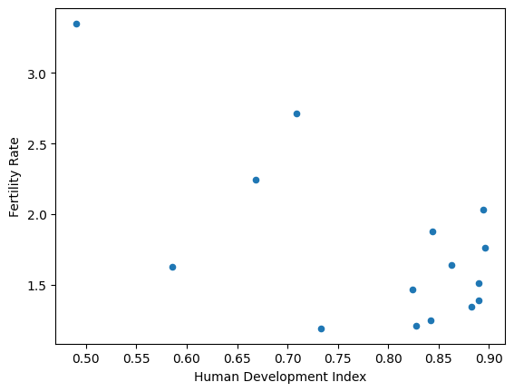
In fact the Pandas .plot methods wrap Matplotlib, so the output from using
Matplotlib directly (see towards the top of this page) will look very similar
to the output from using Pandas .plot, but Pandas can, among other things, use column names to make better default axis labels.