
It’s Pandas time#
We will frequently find ourselves working with data about time. Having a specialised representation of time is useful in numerous respects, primarily because it allows us to do “mathematics with times”. For instance, we may want to use subtraction to calculate the distance between two time points; we cannot do this if we represent dates/times as string data. As such, Python has a useful module for handling dates and times, creatively named “Datetime”.
Python’s Datetimes have a (deserved) reputation for being fiddly (we would wager anyone who has encountered them will agree…). Additionally, in contrast to the close relation between Numpy and Pandas shown on the other pages, the way Pandas handles dates and times is somewhat different to how they are handled in Numpy. To be specific, Pandas stores dates and times using Numpy’s representations, but presents these values to you, dear user, with various attributes that make them look like Python’s Datatimes.
This page will focus on using dates and times as implemented in Pandas. This is also probably the most likely context in which readers will use dates and times…
The page is a brief introduction to Pandas times and dates — there is much more than be done with Pandas dates / times than we will show here - but these are the essentials.
Dates and times in Pandas Series#
First, let’s look at how Pandas handles dates and times. To do this, we’ll create a Pandas Series containing some strings representing dates:
# Our usual imports.
import numpy as np
import pandas as pd
# Create a Series with some strings representing dates
string_time_series = pd.Series(['2025-06-06', '2025-06-07'])
# Show the Series
string_time_series
0    2025-06-06
1    2025-06-07
dtype: str
To no one’s surprise, the type() of these data is str:
# Show the `type()` of the data
first_val = string_time_series.iloc[0]
type(first_val)
str
These representations of dates might look OK at a first glance, but let’s say we want to know the difference in time (duration) between them.
We might surmise that subtracting one date from the other would give us this information.
However, we would be sorely disappointed, when using str data to represent
time:
# Not what we wanted...
second_val = string_time_series.iloc[1]
second_val - first_val
---------------------------------------------------------------------------
TypeError                                 Traceback (most recent call last)
Cell In[4], line 3
      1 # Not what we wanted...
      2 second_val = string_time_series.iloc[1]
----> 3 second_val - first_val

TypeError: unsupported operand type(s) for -: 'str' and 'str'
This is where having a specialized representation of time comes in handy. We
can use the pd.to_datetime() function to convert this data to Pandas’ special
representation of a particular point in time.
Note
Different ways of representing time
As you’ll see below, there are two different and common ways of representing time. These are:
A specific point in time. Pandas represents a specific point in time as a
Timestamp.A duration — for example, the difference in time between two
Timestamps. Pandas represents durations with a type calledTimedelta.
See Pandas timeseries for more.
Let’s convert our string dates to Pandas Timestamps:
# Convert string to time stamps using `to_datetime()`
timestamp_series = pd.to_datetime(string_time_series)
timestamp_series
0   2025-06-06
1   2025-06-07
dtype: datetime64[us]
As you see from the output of the cell above, the dtype of this data is no
longer str (Pandas 3) or object (Pandas 2) as it was above (see Pandas
string in versions 3 and 2. It is now datetime64[ns]
— which we can read as “a datetime representation, in 64 bits, down to the
nanosecond resolution”. Sounds fancy!
We can confirm the type of the data using the type() function:
first_ts_val = timestamp_series.iloc[0]
first_ts_val
Timestamp('2025-06-06 00:00:00')
The Timestamp is Pandas’ special representation of a time point e.g.
a specific point in time. You may wonder why Pandas reports the type() as
a Timestamp but the dtype as datetime64[ns]. For all intents and
purposes, the Timestamp is just a more general description of
datetime64[ns] (with the latter just giving more information about the amount
of memory used for storage and the time resolution…)
We can now do “mathematics with times” and use subtraction to calculate the difference between these dates:
# Get the difference between the two dates
second_ts_val = timestamp_series.iloc[1]
second_ts_val - first_ts_val
Timedelta('1 days 00:00:00')
This operation has returned a Timedelta - the other foundational
representation of time in Pandas. The delta in Timedelta refers to
difference e.g. the difference between two time points. Equally, we can think
of a Timedelta as a representation of a duration (e.g. the duration of time
between two time points).
Pandas helpfully reports that the difference between our two dates is 1 days 00:00:00. You’ll notice here that Pandas made a guess as to the format of the
dates when we created this Series with pd.to_datetime. One could interpret
the original two strings (2025-06-06 and 2025-06-07) are as 6th June 2025
and 7th June 2025, or 6th June 2025 and 6th July 2025. Pandas assumes
that the middle two digits represent months, and this is reasonable, because
this year-first representation is a standard string representation of
time, where the second value is always
the month.
However, more generally, Pandas may or may not be correct in its assumptions.
For example, it is genuinely ambiguous what '06-07-2025 means, because this
could be a North American standard months-days-year string, or a European
standard days-months-year string. In normal contexts, we would need to consult
metadata/documentation associated with our dataset to be sure of the meaning of
the date strings. However, we can control the format with which pd.datetime()
will interpret the date strings, using the format= argument:
# A new Series, using an alternate formatting to the standard Pandas assumes.
other_timestamp_series = pd.to_datetime(string_time_series, format='%Y-%d-%m')
other_timestamp_series
0   2025-06-06
1   2025-07-06
dtype: datetime64[us]
Here we have used the date format string '%Y-%d-%m' as input for the
format= argument. We can read this as “a four digit year, followed by
a hyphen, followed by a two digit day, followed by a hyphen, followed by a two
digit month”.
The, ahem, format of the date format string can take some getting used to. Please see here for the full list of date format options.
We can see that we get a totally different Timedelta when subtracting the
dates interpreted according to the new format:
# Get the difference between the two dates with the alternate formatting
other_timestamp_series.iloc[1] - other_timestamp_series.iloc[0]
Timedelta('30 days 00:00:00')
These two objects (Timestamps and Timedeltas) are the cornerstones of time
representation in Pandas (though there is much else to know about them).
We will look more specifically at the attributes and methods we can use on these representations of time. However, we will do so in the context of Data Frames. As we know, Data Frames are just dictionary-like collections of Series, so any methods/attributes of Data Frame columns can also be used with standalone Series…
Before we move on, it is important to note that pd.to_datetime() can also
convert dates which contain words like the names of months (June, July etc.):
# Representations of dates which contain strings for the names of months (e.g. "JUNE")
a_series_of_str = pd.Series(['2025-JUNE-06', '2025-JUNE-07'])
a_series_of_timestamps = pd.to_datetime(a_series_of_str)
a_series_of_timestamps
/tmp/ipykernel_2832/560003137.py:3: UserWarning: Could not infer format, so each element will be parsed individually, falling back to `dateutil`. To ensure parsing is consistent and as-expected, please specify a format.
  a_series_of_timestamps = pd.to_datetime(a_series_of_str)
0   2025-06-06
1   2025-06-07
dtype: datetime64[us]
Again, Pandas has guessed the format but has implored us to specify the format with which we want the string dates to be interpreted. (Pretty much always, specifying the format is better practice than letting Pandas guess…)
The important point here is that even though the names of months (“JUNE”) went
into the pd.to_datetime() conversion, the Timestamp that came out the other
side contains only numbers. This is important for understanding the essential
nature of Pandas time stamps, as we will see in later sections.
A closer look at time stamps and time deltas#
The Timestamps in the output of the cell above might appear similar to strings, but in terms of the internal representation that Pandas uses they are something entirely different. They are based on something (incredibly sci-fi sounding) called the “Unix Epoch”, to which we will attend later.
To get an insight into this representation, let’s take a closer look at one of the individual Timestamps.
Our variable a_series_of_timestamps is a Pandas Series. As such, as we know
we can use .iloc indexing to retrieve single values from it. In this case, we
retrieve a single Timestamp:
# Retrieve a single Timestamp from the Series
single_timestamp = a_series_of_timestamps.iloc[0]
single_timestamp
Timestamp('2025-06-06 00:00:00')
Attached to any individual Timestamp is an attribute called .value:
# Show the `.value` attribute
single_timestamp.value
1749168000000000000
At first glance this might be confusing - it doesn’t look much like a normal date, or time…
A look through the other attributes reveals more familiarly named units of time. For instance, the year, month and day attributes:
# The `.year` attribute
single_timestamp.year
2025
# The `.month` attribute
single_timestamp.month
6
# The `.day` attribute
single_timestamp.day
6
So what is the mysterious .value attribute?
It is, in fact, more fundamental than the other attributes. It derives from the aforementioned “Unix Epoch”, a slightly ominous sounding name for the duration of time between a given timepoint and a specific timepoint in 1970. Here is an explanation of what that is:
“The Unix epoch is the number of seconds that have elapsed since January 1, 1970 at midnight UTC time minus the leap seconds. This means that at midnight of January 1, 1970, Unix time was 0.” (from https://www.epoch101.com)
The .value attribute reports the number of nanoseconds that have elapsed
between midnight January 1st 1970 and the particular point in time represented
by the Timestamp. This is the fundamental representation that Pandas uses in
Timestamps — the other attributes (year, month, etc) present this
information in a form more understandable to a human.
Why midnight of January 1st 1970? Well we need some point against which to measure other times, and early Unix engineers chose this one. If it isn’t broken why fix it?
Let’s look again at our single Timestamp:
single_timestamp
Timestamp('2025-06-06 00:00:00')
…and then once again at the .value attribute, now we know that it tells us
the number of nanoseconds between our Timestamp and the point where the Unix
Epoch was equal to 0 (midnight, January 1st 1970):
single_timestamp.value
1749168000000000000
To sanity check this, let’s estimate the number of nanoseconds in an average year:
# We've ignored various subtleties here to get an approximate number.
# Taking leap years into account.
average_days_in_year = 365.25
# Days in year * hours in day * minutes in hour * seconds in minute * 1,000,000,000
approx_ns_in_year = average_days_in_year * 24 * 60 * 60 * 1_000_000_000
approx_ns_in_year
3.15576e+16
Thus, if we divide our .value attribute of our Timestamp by approx_ns_in_year we should get something like number of years between the Timestamp and midnight January 1st 1970:
# Calculate the number of years since midnight Jan 1st 1970:
approx_years_since_1_1_1970 = single_timestamp.value / approx_ns_in_year
approx_years_since_1_1_1970
55.42778918548939
55.43 years between the Timestamp (6th June 2025) and January 1st 1970? That sounds about right, but let’s check it by subtracting the rounded approx_years_since_1_1_1970 from our single_timestamp.year, expecting 1970:
single_timestamp.year - np.round(approx_years_since_1_1_1970)
np.float64(1970.0)
Note
Floating point years
We could have subtracted approx_years_since_1_1_1970 from
single_timestamp.year without rounding, and we’d get something midway
through 1969, because approx_years_since_1_1_1970 includes the time from
January 1 2025 to June 6 2025, so subtracting the unrounded value will take us
back to the middle of 1969.
Times and dates in Pandas Data Frames#
Let’s explore Pandas Timestamps further now that we know they are fundamentally a measure of nanoseconds since midnight on 1st January 1970, a duration which can be expressed in more understandable forms like .year, month, day etc. We will again use the Human Development Index dataset. However, to keep things simple, we will just be looking at rows corresponding to Afghanistan:
# Import the dateset
df = pd.read_csv('data/AFG-data-children-per-woman-vs-human-development-index.csv')

df
| Entity | Code | Year | Fertility Rate | Human Development Index | Population | |
|---|---|---|---|---|---|---|
| 0 | Afghanistan | AFG | 1990 | 7.576 | 0.284 | 12045622.0 |
| 1 | Afghanistan | AFG | 1991 | 7.631 | 0.292 | 12238831.0 |
| 2 | Afghanistan | AFG | 1992 | 7.703 | 0.299 | 13278937.0 |
| 3 | Afghanistan | AFG | 1993 | 7.761 | 0.307 | 14943125.0 |
| 4 | Afghanistan | AFG | 1994 | 7.767 | 0.300 | 16250755.0 |
| 5 | Afghanistan | AFG | 1995 | 7.767 | 0.318 | 17065794.0 |
| 6 | Afghanistan | AFG | 1996 | 7.757 | 0.326 | 17763221.0 |
| 7 | Afghanistan | AFG | 1997 | 7.732 | 0.330 | 18452049.0 |
| 8 | Afghanistan | AFG | 1998 | 7.693 | 0.329 | 19159955.0 |
| 9 | Afghanistan | AFG | 1999 | 7.641 | 0.337 | 19887737.0 |
| 10 | Afghanistan | AFG | 2000 | 7.566 | 0.340 | 20130279.0 |
| 11 | Afghanistan | AFG | 2001 | 7.453 | 0.344 | 20284252.0 |
| 12 | Afghanistan | AFG | 2002 | 7.320 | 0.368 | 21378081.0 |
| 13 | Afghanistan | AFG | 2003 | 7.174 | 0.379 | 22733007.0 |
| 14 | Afghanistan | AFG | 2004 | 7.018 | 0.395 | 23560598.0 |
| 15 | Afghanistan | AFG | 2005 | 6.858 | 0.402 | 24404520.0 |
| 16 | Afghanistan | AFG | 2006 | 6.686 | 0.410 | 25424050.0 |
| 17 | Afghanistan | AFG | 2007 | 6.508 | 0.426 | 25909790.0 |
| 18 | Afghanistan | AFG | 2008 | 6.392 | 0.431 | 26482577.0 |
| 19 | Afghanistan | AFG | 2009 | 6.295 | 0.441 | 27466056.0 |
| 20 | Afghanistan | AFG | 2010 | 6.195 | 0.449 | 28284036.0 |
| 21 | Afghanistan | AFG | 2011 | 6.094 | 0.457 | 29347668.0 |
| 22 | Afghanistan | AFG | 2012 | 5.985 | 0.467 | 30559988.0 |
| 23 | Afghanistan | AFG | 2013 | 5.879 | 0.475 | 31622662.0 |
| 24 | Afghanistan | AFG | 2014 | 5.770 | 0.480 | 32792472.0 |
| 25 | Afghanistan | AFG | 2015 | 5.652 | 0.479 | 33831716.0 |
| 26 | Afghanistan | AFG | 2016 | 5.542 | 0.483 | 34700565.0 |
| 27 | Afghanistan | AFG | 2017 | 5.433 | 0.485 | 35688889.0 |
| 28 | Afghanistan | AFG | 2018 | 5.327 | 0.486 | 36742997.0 |
| 29 | Afghanistan | AFG | 2019 | 5.238 | 0.492 | 37856071.0 |
| 30 | Afghanistan | AFG | 2020 | 5.145 | 0.488 | 39068933.0 |
| 31 | Afghanistan | AFG | 2021 | 5.039 | 0.473 | 40000360.0 |
| 32 | Afghanistan | AFG | 2022 | 4.932 | 0.462 | 40578801.0 |
If you look at the Year column, you can see that what we have is a running set of observations (all from Afghanistan) from the year 1990 up until the year 2022.
This sort of data - a series of observations over time - is called time series data. In fact, the name of Pandas Series comes from “time series”, as this is the sort of data the library was originally designed to be used with.
Here we have one observational unit (in this case a country), measured over time on the same variables. If we have data like this, then we can use a useful trick to inspect all time-related trends at once.
We just call the .plot() method on the whole Data Frame, using the subplots=True argument), and we get the following neat result:
# A useful trick to time-series data!
df.plot(subplots=True);
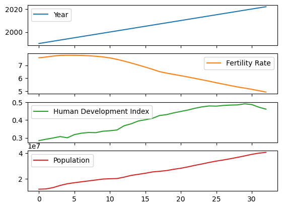
As expected, the trend for Year increasely linearly (duh!), whilst Fertility Rate falls and Human Development Index/Population (mostly) climb.
We are undoubtedly viewing time-rleated trends here, but we are doing so based on a non-specialized representation of the times in the Year column:
# What type of data is in the `Year` column?
df['Year'].dtype
dtype('int64')
Because the Year formats in this dataset, unlike the str dates we used earlier, do NOT contain anything string specific (hyphens and the like), Pandas has interpreted them as int data.
# Inspect the `Year` column
df['Year']
0     1990
1     1991
2     1992
3     1993
4     1994
5     1995
6     1996
7     1997
8     1998
9     1999
10    2000
11    2001
12    2002
13    2003
14    2004
15    2005
16    2006
17    2007
18    2008
19    2009
20    2010
21    2011
22    2012
23    2013
24    2014
25    2015
26    2016
27    2017
28    2018
29    2019
30    2020
31    2021
32    2022
Name: Year, dtype: int64
This is OK as far as it goes, but we can do better.
Let’s convert the Year values to Timestamp data, to see the host of
time-specific attributes and methods that we then get access to.
NB: we will call the column containing the Timestamps Year_as_Timestamp, and
rename the original Year column to Year_as_string to avoid confusion:
# Rename the `Year` column
df = df.rename(columns={'Year': 'Year_as_string'})

# Convert the month data to Timestamp.
df['Year_as_Timestamp'] = pd.to_datetime(df['Year_as_string'], format='%Y')
df['Year_as_Timestamp']
0    1990-01-01
1    1991-01-01
2    1992-01-01
3    1993-01-01
4    1994-01-01
5    1995-01-01
6    1996-01-01
7    1997-01-01
8    1998-01-01
9    1999-01-01
10   2000-01-01
11   2001-01-01
12   2002-01-01
13   2003-01-01
14   2004-01-01
15   2005-01-01
16   2006-01-01
17   2007-01-01
18   2008-01-01
19   2009-01-01
20   2010-01-01
21   2011-01-01
22   2012-01-01
23   2013-01-01
24   2014-01-01
25   2015-01-01
26   2016-01-01
27   2017-01-01
28   2018-01-01
29   2019-01-01
30   2020-01-01
31   2021-01-01
32   2022-01-01
Name: Year_as_Timestamp, dtype: datetime64[us]
Here we used a much simpler time stamp format string ('%Y') for the format=
argument. We can just read the string as “a four digit representation of
year” (e.g. 1990).
You’ll see in the output of the cell above that Pandas has added a month and
a day to the original Year_as_string values. This is because Pandas
Timestamps represent a specific time point - so a whole year is too low of
a resolution for this representation of time. As a result, Pandas has
automatically chosen January 1st to flesh out the time point.
For most purposes this addition is fine. It might create problems if we mix this data with other time-related data which is higher-resolution than “year”, but for our present purpose we are not going to do that, so let’s just let Pandas make this harmless addition, as it gives us the benefit of a specialized representation of time, which we will see in the next section.
The .dt accessor#
Relative to representing time with str or int data, Pandas Timestamps contain many attributes which represent specific units of time.
Let’s look at just one value from the Year_as_Timestamp column:
# A look at a specific time stamp.
first_year_ts = df['Year_as_Timestamp'].iloc[0]
first_year_ts
Timestamp('1990-01-01 00:00:00')
We can read the numbers in the parentheses as “0 minutes, 0 seconds past midnight on 1st January 1990”.
Let’s try to index further into the Timestamp:
# Oh no....
first_year_ts[0]
---------------------------------------------------------------------------
TypeError                                 Traceback (most recent call last)
Cell In[27], line 2
      1 # Oh no....
----> 2 first_year_ts[0]

TypeError: 'Timestamp' object is not subscriptable
This inability to index (using integers) into the Timestamp might seem frustrating, but it is sensible. The underlying representation is a single number, so indexing into a number does not make sense. One could also think of the Timestamp value as something from which one could retrieve information like year, month or day, but it’s not clear what [0] would mean in terms of — for example — year, month or day.
Conversely, remember the advantages of using index labels vs integer
indexes? These include greater human interpretability,
less temptation to error (which derived value does [0] refer to).
Well, Pandas’ representation of time has the same advantages. To retrieve more
specific aspects of the Timestamp we must use meaningful, readable and
hard to misinterpret attribute names.
We can access these time-specific attributes via the .dt. accessor (read as
“datetime”, a synonym for Timestamp). Much like the .str. accessor we saw
earlier this is an accessor specialized for
a specific data type, in this case Timestamp data.
As with the .str accessor, the .dt. accessor operates on all values of a Data Frame column (Pandas Series) in parallel.
For instance, to grab just the year information, we can use .dt.year:
# View the `year` attribute
df['Year_as_Timestamp'].dt.year
0     1990
1     1991
2     1992
3     1993
4     1994
5     1995
6     1996
7     1997
8     1998
9     1999
10    2000
11    2001
12    2002
13    2003
14    2004
15    2005
16    2006
17    2007
18    2008
19    2009
20    2010
21    2011
22    2012
23    2013
24    2014
25    2015
26    2016
27    2017
28    2018
29    2019
30    2020
31    2021
32    2022
Name: Year_as_Timestamp, dtype: int32
To get this information for a specific row, we can just chain on an .iloc indexing operation:
df['Year_as_Timestamp'].dt.year.iloc[0]
np.int32(1990)
We can use other clearly named attributes, accessing time-based information down to the smallest unit of time represented in the Timestamp.
We will go through these in order (.dt.month, .dt.day, .dt.hour, .dt.minute, .dt.second) in the cells below:
# View the `month` attribute (which here has been automatically set to 1 by Pandas)
df['Year_as_Timestamp'].dt.month
0     1
1     1
2     1
3     1
4     1
5     1
6     1
7     1
8     1
9     1
10    1
11    1
12    1
13    1
14    1
15    1
16    1
17    1
18    1
19    1
20    1
21    1
22    1
23    1
24    1
25    1
26    1
27    1
28    1
29    1
30    1
31    1
32    1
Name: Year_as_Timestamp, dtype: int32
# View the `day` attribute (which here has been automatically set to 1 by Pandas)
df['Year_as_Timestamp'].dt.day
0     1
1     1
2     1
3     1
4     1
5     1
6     1
7     1
8     1
9     1
10    1
11    1
12    1
13    1
14    1
15    1
16    1
17    1
18    1
19    1
20    1
21    1
22    1
23    1
24    1
25    1
26    1
27    1
28    1
29    1
30    1
31    1
32    1
Name: Year_as_Timestamp, dtype: int32
# View the `hour` attribute (which here has been automatically set to 0 by Pandas)
df['Year_as_Timestamp'].dt.hour
0     0
1     0
2     0
3     0
4     0
5     0
6     0
7     0
8     0
9     0
10    0
11    0
12    0
13    0
14    0
15    0
16    0
17    0
18    0
19    0
20    0
21    0
22    0
23    0
24    0
25    0
26    0
27    0
28    0
29    0
30    0
31    0
32    0
Name: Year_as_Timestamp, dtype: int32
# View the `minute` attribute (which here has been automatically set to 0 by Pandas)
df['Year_as_Timestamp'].dt.minute
0     0
1     0
2     0
3     0
4     0
5     0
6     0
7     0
8     0
9     0
10    0
11    0
12    0
13    0
14    0
15    0
16    0
17    0
18    0
19    0
20    0
21    0
22    0
23    0
24    0
25    0
26    0
27    0
28    0
29    0
30    0
31    0
32    0
Name: Year_as_Timestamp, dtype: int32
# View the `second` attribute (which here has been automatically set to 0 by Pandas)
df['Year_as_Timestamp'].dt.second
0     0
1     0
2     0
3     0
4     0
5     0
6     0
7     0
8     0
9     0
10    0
11    0
12    0
13    0
14    0
15    0
16    0
17    0
18    0
19    0
20    0
21    0
22    0
23    0
24    0
25    0
26    0
27    0
28    0
29    0
30    0
31    0
32    0
Name: Year_as_Timestamp, dtype: int32
We can see that the sequence with which we just “walked” through the .dt. attributes (.dt.month, .dt.day, .dt.hour, .dt.minute, .dt.second) corresponds to the order of the output of a single Timestamp:
# View an individual Timestamp
df['Year_as_Timestamp'].iloc[0]
Timestamp('1990-01-01 00:00:00')
Timestamps provide a structured, easy to access and hard to misinterpret, representation of time, fundamentally based on the Unix Epoch (the distance between a particular timepoint and midnight January 1st 1970).
From this nanosecond representation each attribute converts the .value into a more human-interpretable unit of time. This is all Timestamps in Pandas are!
We mentioned earlier than the names of months (like “June”/”July” etc, as well as other string-y stuff) can go into a pd.to_datetime() conversion, but the result will always contain only numbers. These numbers are stored in a sequence of attributes which represent increasingly smaller units of time (year, month, day, minute, second etc.) as numbers, even if the original input containing strings like “June”, “July” etc.
Using the .dt. accessor, we can easily do things like filter our a specific year using these attributes:
# Filter using a Boolean array from the `.dt` accessor
df[df['Year_as_Timestamp'].dt.year == 1990]
| Entity | Code | Year_as_string | Fertility Rate | Human Development Index | Population | Year_as_Timestamp | |
|---|---|---|---|---|---|---|---|
| 0 | Afghanistan | AFG | 1990 | 7.576 | 0.284 | 12045622.0 | 1990-01-01 |
See further methods and attributes available from the .dt. accessor here.
Using Timestamps in a Data Frame index#
Now we have our special time representations, a real strength of having them is to put them in the index of the Data Frame. This let’s us easily do some useful things, like slicing the Data Frame rows by time.
We can do this using the previously seen .set_index() method:
# Put Timestamps in the index
df = df.set_index('Year_as_Timestamp')

df
| Entity | Code | Year_as_string | Fertility Rate | Human Development Index | Population | |
|---|---|---|---|---|---|---|
| Year_as_Timestamp | ||||||
| 1990-01-01 | Afghanistan | AFG | 1990 | 7.576 | 0.284 | 12045622.0 |
| 1991-01-01 | Afghanistan | AFG | 1991 | 7.631 | 0.292 | 12238831.0 |
| 1992-01-01 | Afghanistan | AFG | 1992 | 7.703 | 0.299 | 13278937.0 |
| 1993-01-01 | Afghanistan | AFG | 1993 | 7.761 | 0.307 | 14943125.0 |
| 1994-01-01 | Afghanistan | AFG | 1994 | 7.767 | 0.300 | 16250755.0 |
| 1995-01-01 | Afghanistan | AFG | 1995 | 7.767 | 0.318 | 17065794.0 |
| 1996-01-01 | Afghanistan | AFG | 1996 | 7.757 | 0.326 | 17763221.0 |
| 1997-01-01 | Afghanistan | AFG | 1997 | 7.732 | 0.330 | 18452049.0 |
| 1998-01-01 | Afghanistan | AFG | 1998 | 7.693 | 0.329 | 19159955.0 |
| 1999-01-01 | Afghanistan | AFG | 1999 | 7.641 | 0.337 | 19887737.0 |
| 2000-01-01 | Afghanistan | AFG | 2000 | 7.566 | 0.340 | 20130279.0 |
| 2001-01-01 | Afghanistan | AFG | 2001 | 7.453 | 0.344 | 20284252.0 |
| 2002-01-01 | Afghanistan | AFG | 2002 | 7.320 | 0.368 | 21378081.0 |
| 2003-01-01 | Afghanistan | AFG | 2003 | 7.174 | 0.379 | 22733007.0 |
| 2004-01-01 | Afghanistan | AFG | 2004 | 7.018 | 0.395 | 23560598.0 |
| 2005-01-01 | Afghanistan | AFG | 2005 | 6.858 | 0.402 | 24404520.0 |
| 2006-01-01 | Afghanistan | AFG | 2006 | 6.686 | 0.410 | 25424050.0 |
| 2007-01-01 | Afghanistan | AFG | 2007 | 6.508 | 0.426 | 25909790.0 |
| 2008-01-01 | Afghanistan | AFG | 2008 | 6.392 | 0.431 | 26482577.0 |
| 2009-01-01 | Afghanistan | AFG | 2009 | 6.295 | 0.441 | 27466056.0 |
| 2010-01-01 | Afghanistan | AFG | 2010 | 6.195 | 0.449 | 28284036.0 |
| 2011-01-01 | Afghanistan | AFG | 2011 | 6.094 | 0.457 | 29347668.0 |
| 2012-01-01 | Afghanistan | AFG | 2012 | 5.985 | 0.467 | 30559988.0 |
| 2013-01-01 | Afghanistan | AFG | 2013 | 5.879 | 0.475 | 31622662.0 |
| 2014-01-01 | Afghanistan | AFG | 2014 | 5.770 | 0.480 | 32792472.0 |
| 2015-01-01 | Afghanistan | AFG | 2015 | 5.652 | 0.479 | 33831716.0 |
| 2016-01-01 | Afghanistan | AFG | 2016 | 5.542 | 0.483 | 34700565.0 |
| 2017-01-01 | Afghanistan | AFG | 2017 | 5.433 | 0.485 | 35688889.0 |
| 2018-01-01 | Afghanistan | AFG | 2018 | 5.327 | 0.486 | 36742997.0 |
| 2019-01-01 | Afghanistan | AFG | 2019 | 5.238 | 0.492 | 37856071.0 |
| 2020-01-01 | Afghanistan | AFG | 2020 | 5.145 | 0.488 | 39068933.0 |
| 2021-01-01 | Afghanistan | AFG | 2021 | 5.039 | 0.473 | 40000360.0 |
| 2022-01-01 | Afghanistan | AFG | 2022 | 4.932 | 0.462 | 40578801.0 |
If we view the index, Pandas will helpfully reveal that setting Year as the index - a column which contained only Timestamps - has created a DatetimeIndex. As the name might reveal, this is an index containing only Timestamps (aka dates / times):
# Show the index
df.index
DatetimeIndex(['1990-01-01', '1991-01-01', '1992-01-01', '1993-01-01',
               '1994-01-01', '1995-01-01', '1996-01-01', '1997-01-01',
               '1998-01-01', '1999-01-01', '2000-01-01', '2001-01-01',
               '2002-01-01', '2003-01-01', '2004-01-01', '2005-01-01',
               '2006-01-01', '2007-01-01', '2008-01-01', '2009-01-01',
               '2010-01-01', '2011-01-01', '2012-01-01', '2013-01-01',
               '2014-01-01', '2015-01-01', '2016-01-01', '2017-01-01',
               '2018-01-01', '2019-01-01', '2020-01-01', '2021-01-01',
               '2022-01-01'],
              dtype='datetime64[us]', name='Year_as_Timestamp', freq=None)
# Show the `type()` of the index
type(df.index)
pandas.DatetimeIndex
# Show an individual Timestamp from the `index`
df.index[0]
Timestamp('1990-01-01 00:00:00')
We can get the aforementioned benefits of .loc
indexing on our Timestamps.
For instance, we can .loc index just data from the year 1990:
# Using `.loc` with a year
df.loc["1990"]
| Entity | Code | Year_as_string | Fertility Rate | Human Development Index | Population | |
|---|---|---|---|---|---|---|
| Year_as_Timestamp | ||||||
| 1990-01-01 | Afghanistan | AFG | 1990 | 7.576 | 0.284 | 12045622.0 |
We can also do neat slicing operations using time information. For instance showing all rows corresponding to years between 1990 and 1995:
# Slice the years using `.loc`
df.loc["1990" : "1995"]
| Entity | Code | Year_as_string | Fertility Rate | Human Development Index | Population | |
|---|---|---|---|---|---|---|
| Year_as_Timestamp | ||||||
| 1990-01-01 | Afghanistan | AFG | 1990 | 7.576 | 0.284 | 12045622.0 |
| 1991-01-01 | Afghanistan | AFG | 1991 | 7.631 | 0.292 | 12238831.0 |
| 1992-01-01 | Afghanistan | AFG | 1992 | 7.703 | 0.299 | 13278937.0 |
| 1993-01-01 | Afghanistan | AFG | 1993 | 7.761 | 0.307 | 14943125.0 |
| 1994-01-01 | Afghanistan | AFG | 1994 | 7.767 | 0.300 | 16250755.0 |
| 1995-01-01 | Afghanistan | AFG | 1995 | 7.767 | 0.318 | 17065794.0 |
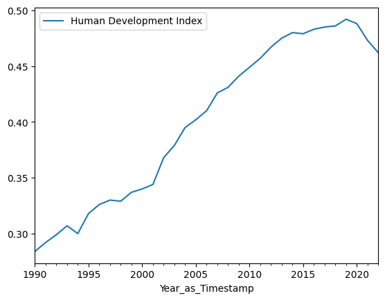
Simple calls to the .plot() method (using the y= argument only) will now
automatically place the Timestamp information on the x-axis:
# Plotting will automatically use the time stamp index on the x-axis
df.plot(y='Human Development Index');
Summary#
There is a lot more would could say about dates and times (both in Pandas and in general), but that is enough for this brief introduction.
The key points are:
Pandas Timestamps are values that represent points in time. The Pandas API allows us to get different units of time from these values, such as year, month, day, hour, minute and so on.
Pandas Timedeltas are values that represent durations.
Timestamps and Timedeltas let us do “mathematics with times” which we cannot do with string representations.
Putting Timestamps in our index allows for some neat indexing and plotting operations.